4.1 — Modeling Firms With Market Power — Appendix
Monopolists Only Produce Where Demand is Elastic: Proof
Let’s first show the relationship between
Remember, we’ve simplified
Now that we have this alternate expression for
I rearrange the last line only to remind us that
Now note the following:
- If
- If
- If
Hence, a monopolist will never produce in the inelastic region of the demand curve (where
See the graphs on slide 33.
Derivation of the Lerner Index
Marginal revenue is strongly related to the price elasticity of demand, which is
We derived marginal revenue (in the slides) as:
Firms will always maximize profits where:
The left side gives us the fraction of price that is markup
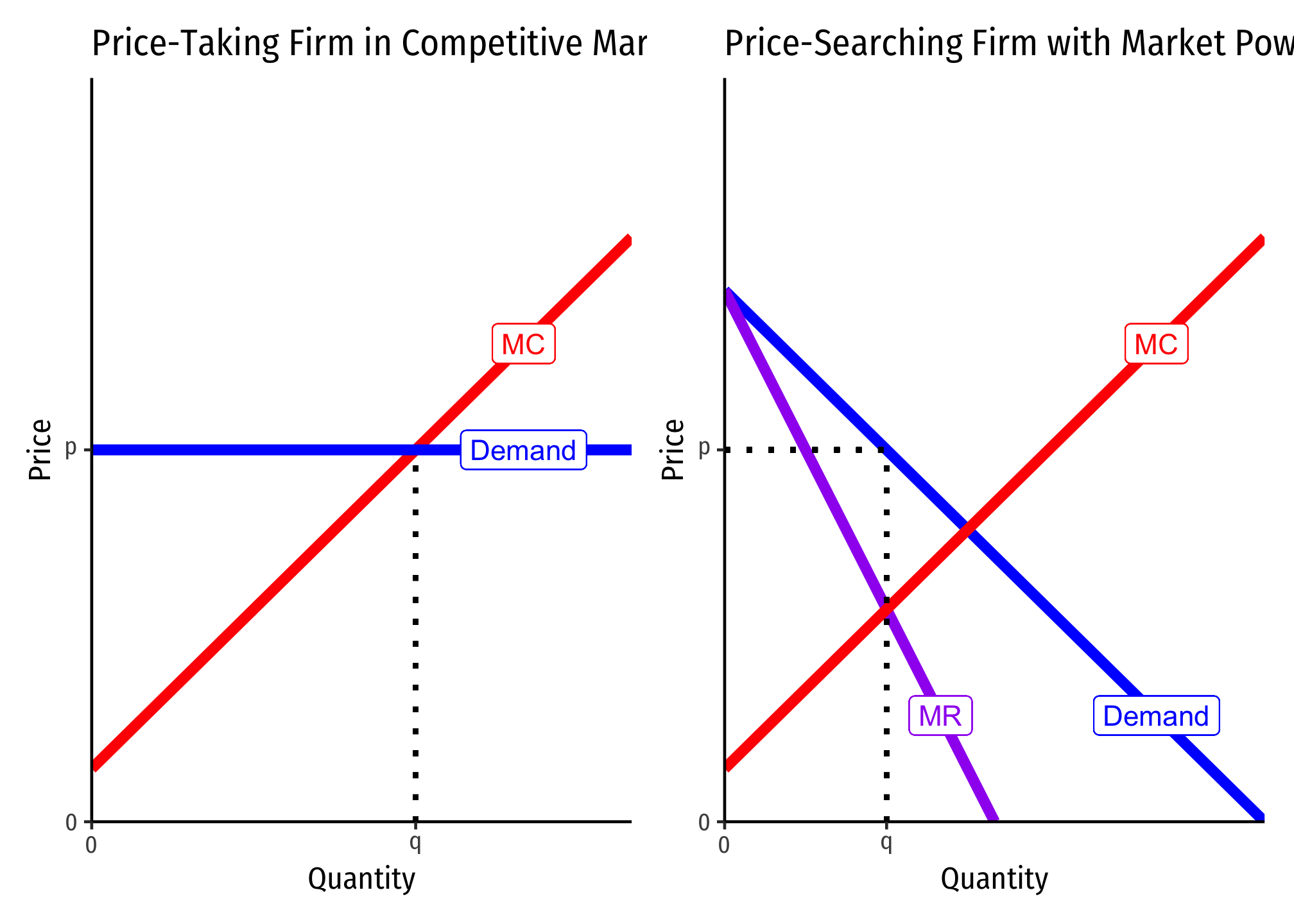
Firms With Market Power vs. Competitive Firms’ Responses to Market Changes
Consider a firm in a competitive market (left) and a firm with market power (right):
An Increase in Firms’ Marginal Cost
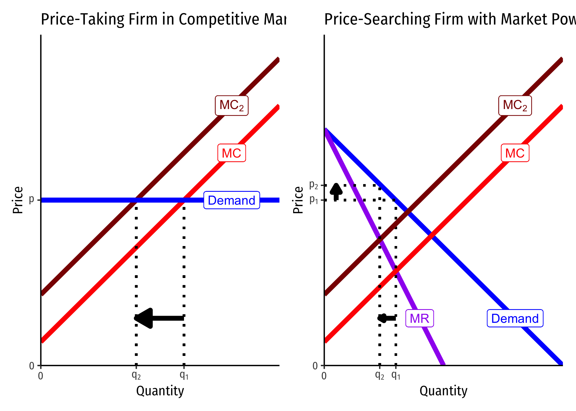
A competitive firm responds by only changing its output
A Shift in Market Demand
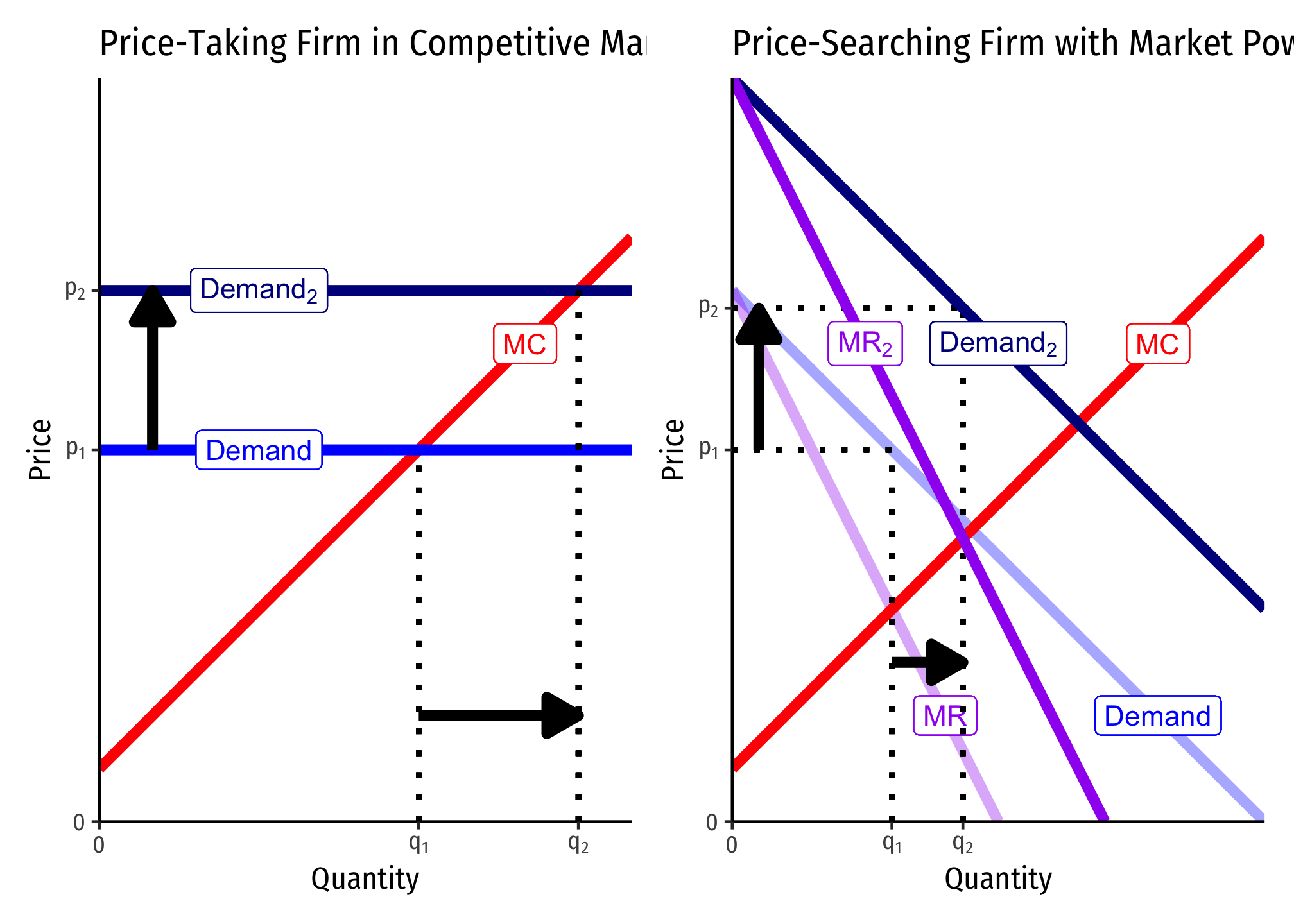
Both firms change
A Change in Price Elasticity of Demand
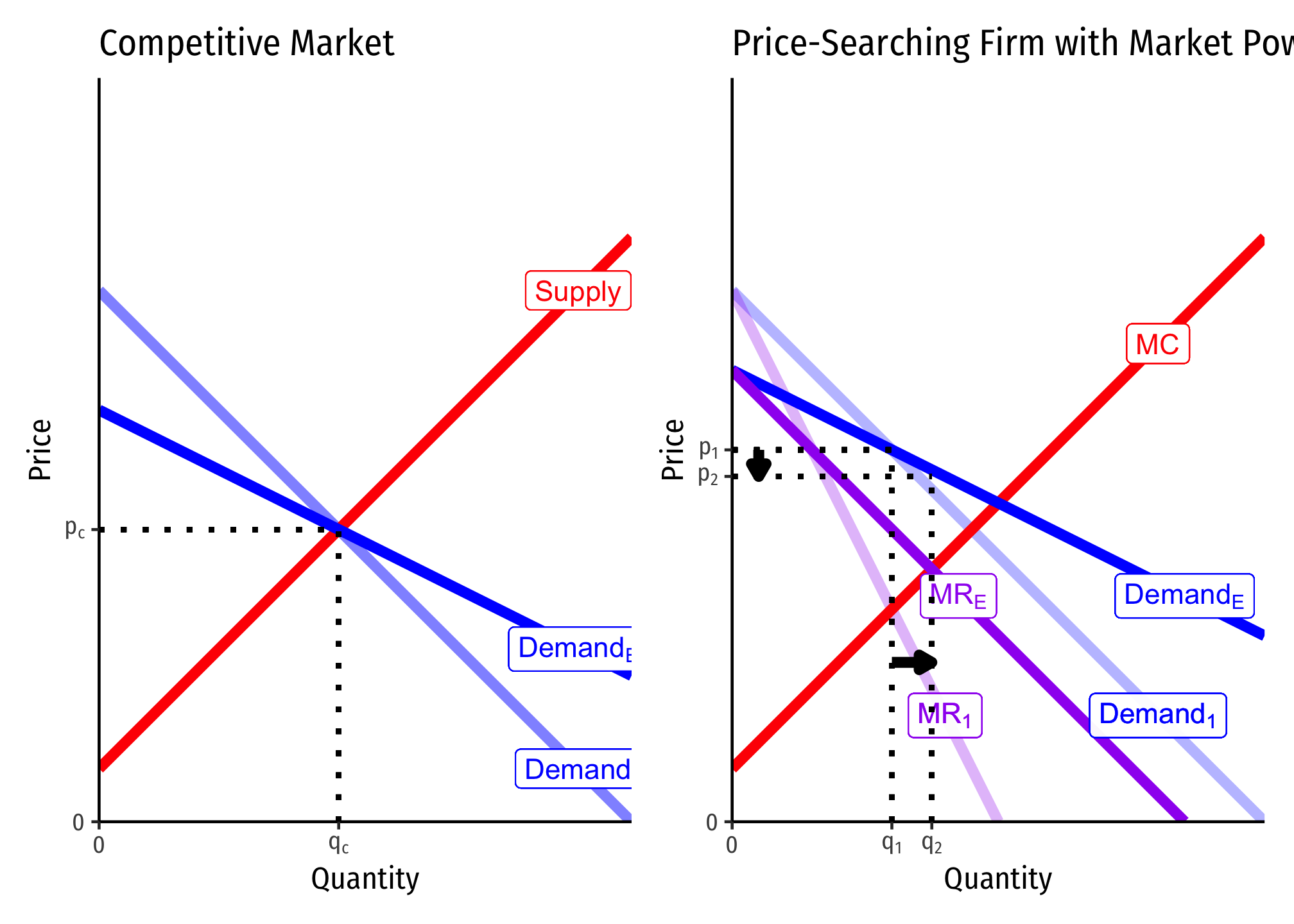
For the competitive market on the left, there is no change in
Footnotes
I sometimes simplify it as