1.6 — Income & Substitution Effects
ECON 306 • Microeconomic Analysis • Fall 2022
Ryan Safner
Associate Professor of Economics
safner@hood.edu
ryansafner/microF22
microF22.classes.ryansafner.com
A Demand Function (Again)
- A consumer’s demand (for good x) depends on current prices & income:
qDx=qDx(m,px,py)
- How does demand (for x) change?
- Income effects (ΔqDxΔm): how qDx changes with changes in income
- Cross-price effects (ΔqDxΔpy): how qDx changes with changes in prices of other goods (e.g. y)
- (Own) Price effects (ΔqDxΔpx): how qDx changes with changes in price (of x)

The (Own) Price Effect
The (Own) Price Effect
- Price effect: change in optimal consumption of a good associated with a change in its price, holding income and other prices constant
ΔqDxΔpx<0
The law of demand: as the price of a good rises, people will tend to buy less of that good (and vice versa)
- i.e. the price effect is negative!

Decomposing the Price Effect
The price effect (law of demand) is actually the net result of two effects
Decomposing the Price Effect
The price effect (law of demand) is actually the net result of two effects
- (Real) income effect: change in consumption due to change in real purchasing power
Decomposing the Price Effect
The price effect (law of demand) is actually the net result of two effects
(Real) income effect: change in consumption due to change in real purchasing power
Substitution effect: change in consumption due to change in relative prices
Decomposing the Price Effect
The price effect (law of demand) is actually the net result of two effects
(Real) income effect: change in consumption due to change in real purchasing power
Substitution effect: change in consumption due to change in relative prices
Price Effect = Real income effect + Substitution Effect
(Real) Income Effect
(Real) Income Effect: Demonstration
Suppose there is only 1 good to consume, x. You have a $100 income, and the price of x is $10. You consume 10 units of x
Suppose the price of x rises to $20. You now consume 5 units of x.
This is the real income effect

(Real) Income Effect: Demonstration
Real income effect: your consumption mix changes because of the change in the price of x changes your real income or purchasing power (the amount of goods you can buy)
Note your actual (nominal) income ($100) never changed!

(Real) Income Effect: Size
The size of the income effect depends on how large a portion of your budget you spend on the good
Large-budget items:
- e.g. Housing/apartment rent, car prices
- Price increase/decreases makes you much poorer/wealthier

(Real) Income Effect: Size
The size of the income effect depends on how large a portion of your budget you spend on the good
Small-budget items:
- e.g. pencils, toothpicks, candy
- Price changes don’t have much of an effect on your wealth or change your behavior much

Substitution Effect
Substitution Effect: Demonstration
Suppose there are 1000’s of goods, none of them a major part of your budget
- So real income effect is insignificant
Suppose the price of good x increases
You would consume less of x relative to other goods because x is now relatively more expensive
That’s the substitution effect

Substitution Effect: Demonstration
Substitution effect: consumption mix changes because of a change in relative prices
Buy more of the (now) relatively cheaper items
Buy less of the (now) relatively more expensive item (x)

Putting the Effects Together
Putting the Effects Together
- Real income effect: change in consumption due to change in real purchasing power
- Could go in different directions: positive (normal goods) or negative (inferior goods)
- Higher price of x means you must buy less x, y, or both (depending on your preferences)
Putting the Effects Together
- Real income effect: change in consumption due to change in real purchasing power
- Could go in different directions: positive (normal goods) or negative (inferior goods)
- Higher price of x means you must buy less x, y, or both (depending on your preferences)
- Substitution effect: change in consumption due to change in relative prices
- If x gets more expensive relative to y, consume ↓x (and ↑y)
- Always the same direction: (↓ relatively expensive goods, ↑ relatively cheaper goods)
- This is why demand curves slope downwards!
Price Effect = Real income effect + Substitution Effect
Real Income and Substitution Effects, Graphically I
- Original optimal consumption (A)

Real Income and Substitution Effects, Graphically I
Original optimal consumption (A)
(Total) price effect: A→C
Let's decompose this into the two effects

Real Income and Substitution Effects, Graphically II
- Substitution effect: what you would choose under the new exchange rate to remain indifferent as before the change

Real Income and Substitution Effects, Graphically II
Substitution effect: what you would choose under the new exchange rate to remain indifferent as before the change
Graphically: shift new budget constraint inwards until tangent with old indifference curve
A→B on same I.C. (↓ x, ↑ y)
- Note: Point B must be a different point on the original curve! Why?

Real Income and Substitution Effects, Graphically III
- (Real) income effect: change in consumption due to the change in purchasing power from the price change

Real Income and Substitution Effects, Graphically III
(Real) income effect: change in consumption due to the change in purchasing power from the price change
B→C to new budget constraint (can buy less of x and/or y)
Real Income and Substitution Effects, Graphically IV
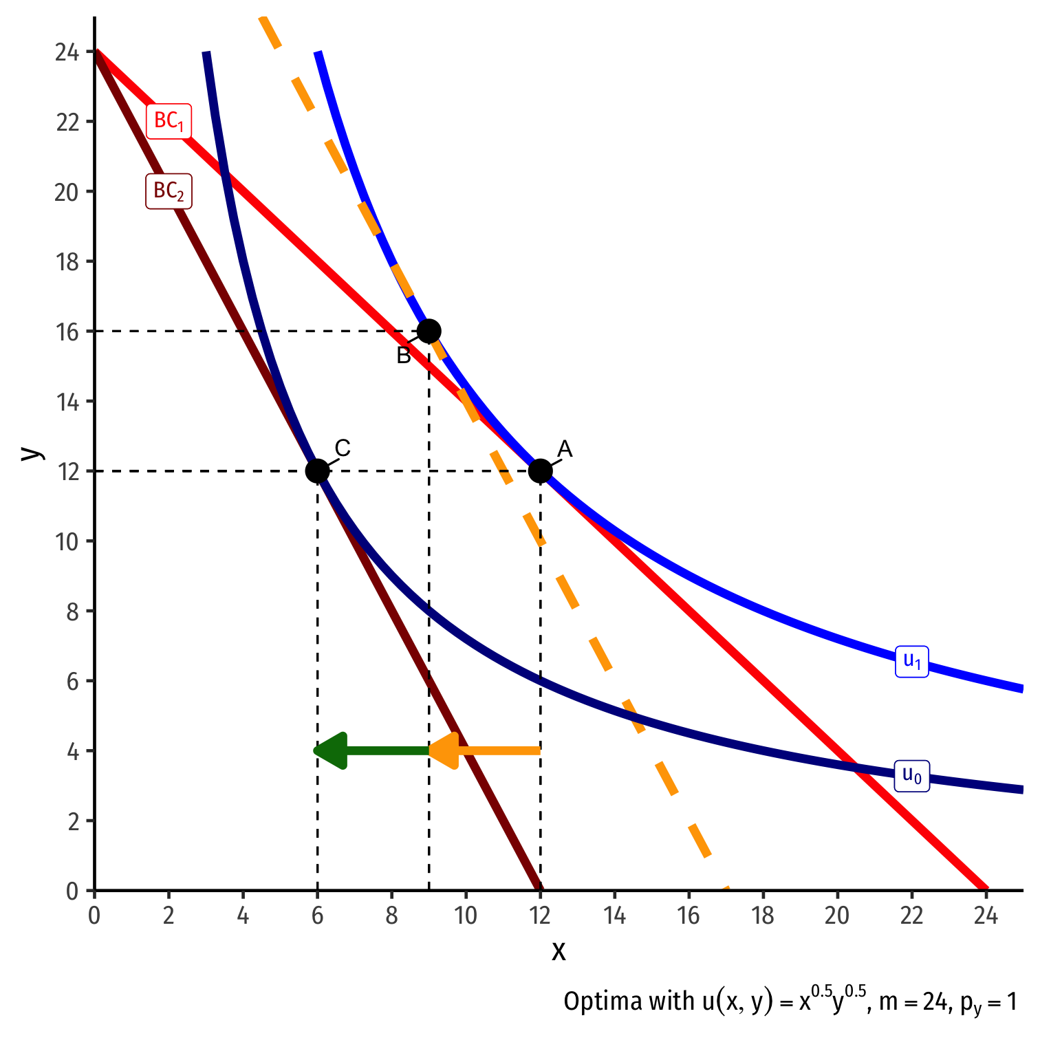
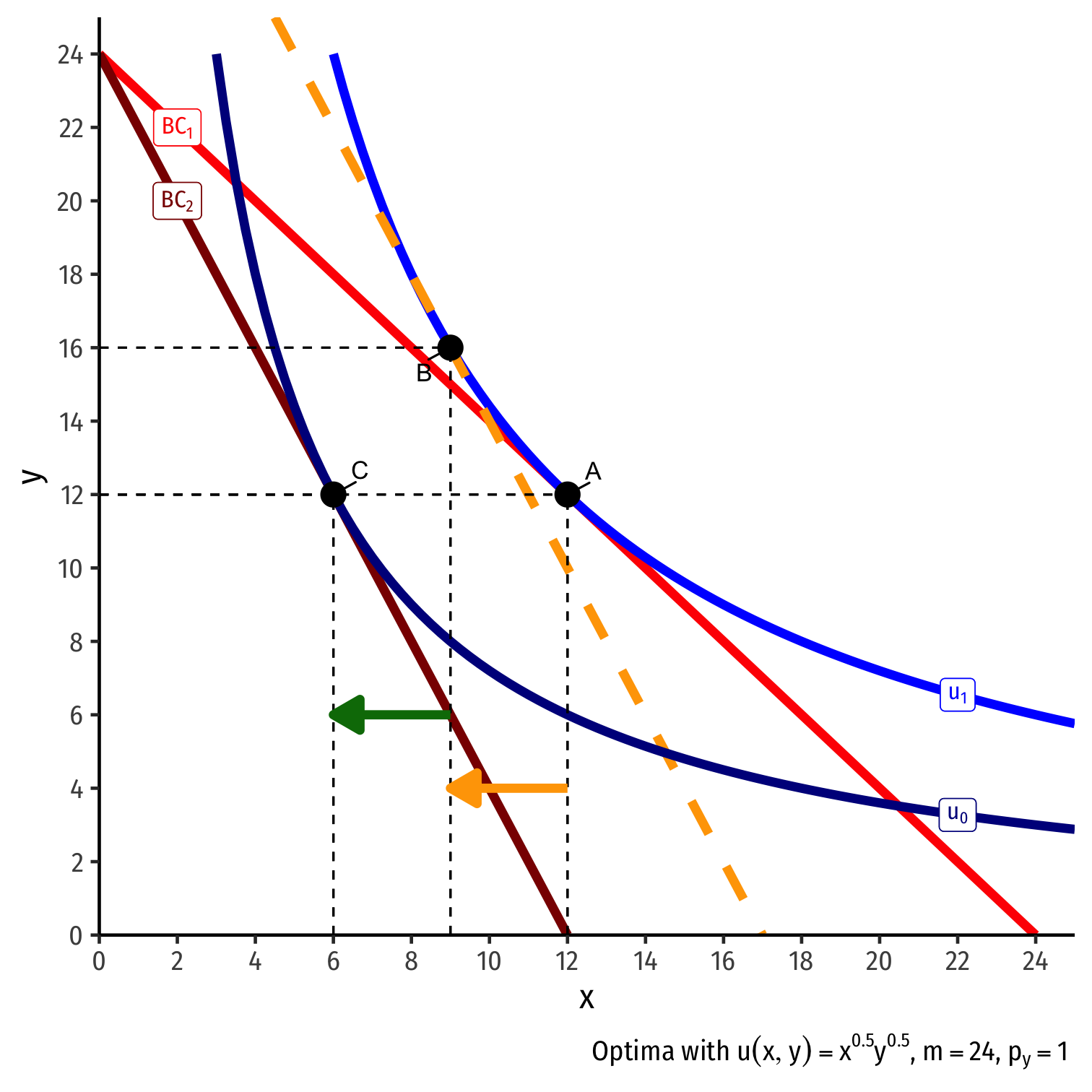
- Original optimal consumption (A)

Real Income and Substitution Effects, Graphically IV
Original optimal consumption (A)
Price of x rises, new optimal consumption at (C)
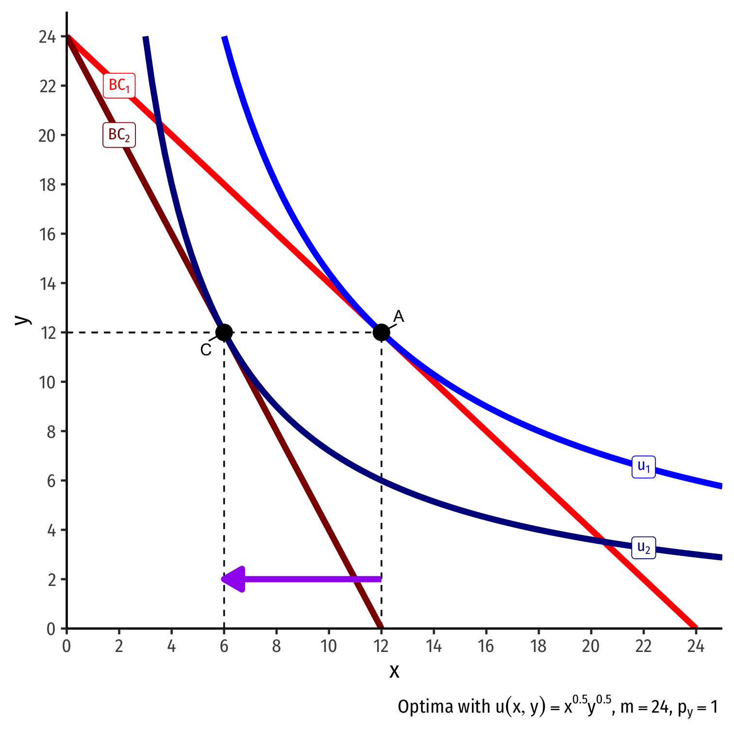
Real Income and Substitution Effects, Graphically IV
Original optimal consumption (A)
Price of x rises, new optimal consumption at (C)
Substitution effect: A→B on same I.C. (↓ more expensive x and ↑ y)
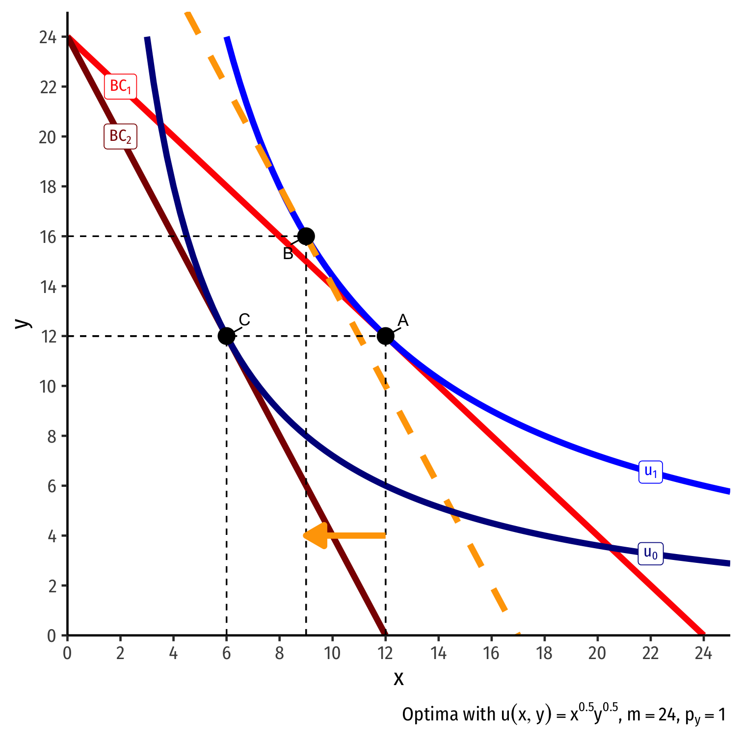
Real Income and Substitution Effects, Graphically IV
Original optimal consumption (A)
Price of x rises, new optimal consumption at (C)
Substitution effect: A→B on same I.C. (↓ more expensive x and ↑ y)
(Real) income effect: B→C to new budget constraint (can buy less of x and/or y)
Real Income and Substitution Effects, Graphically IV
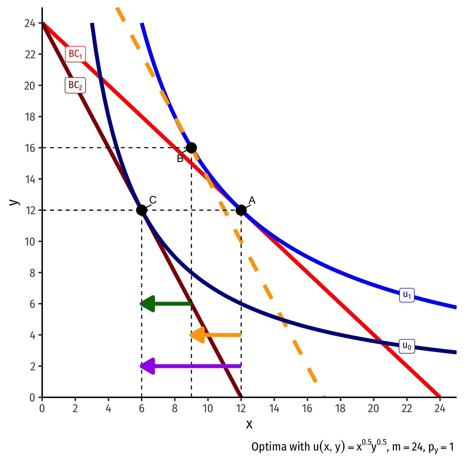
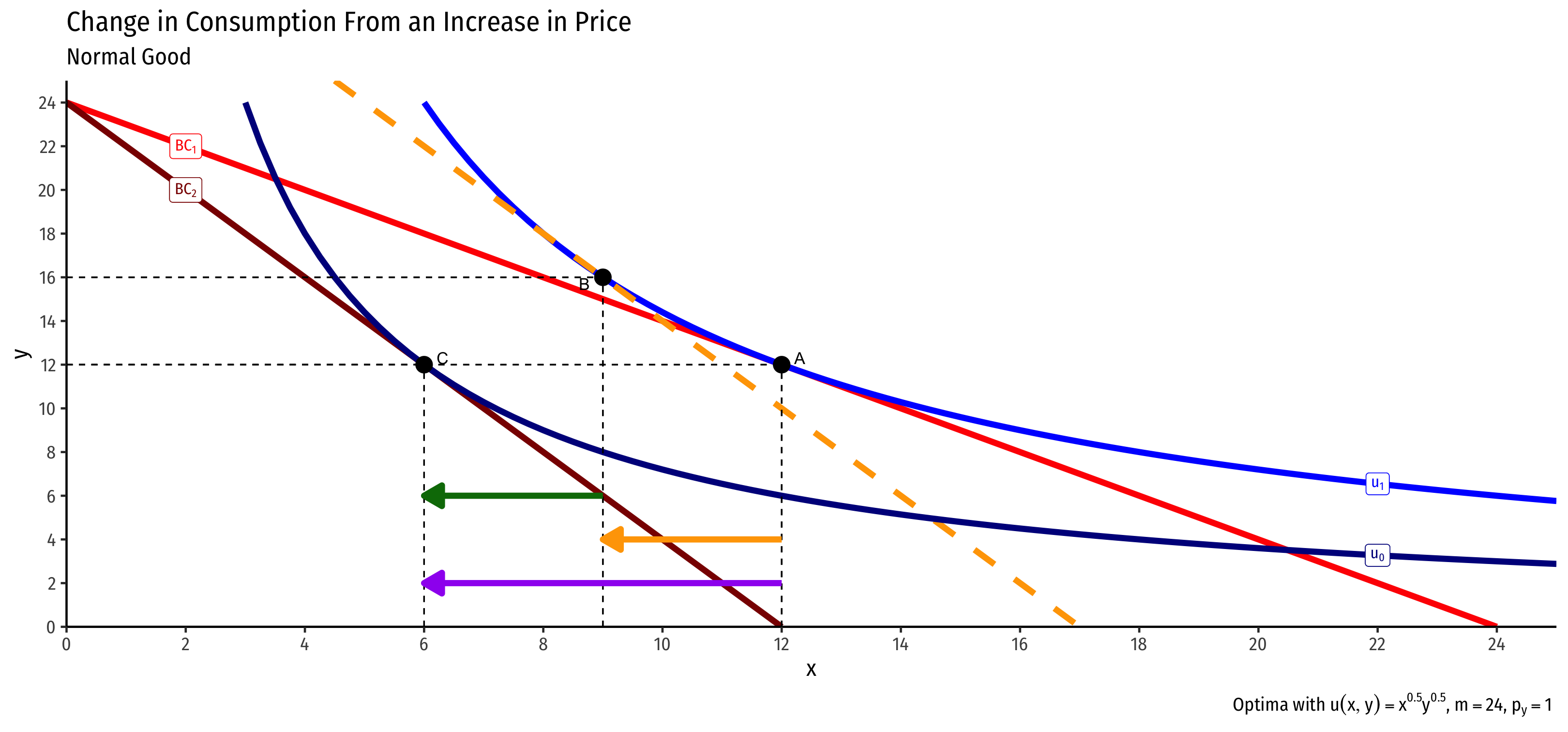
Original optimal consumption (A)
Price of x rises, new optimal consumption at (C)
Substitution effect: A→B on same I.C. (↓ more expensive x and ↑ y)
(Real) income effect: B→C to new budget constraint (can buy less of x and/or y)
(Total) price effect: A→C
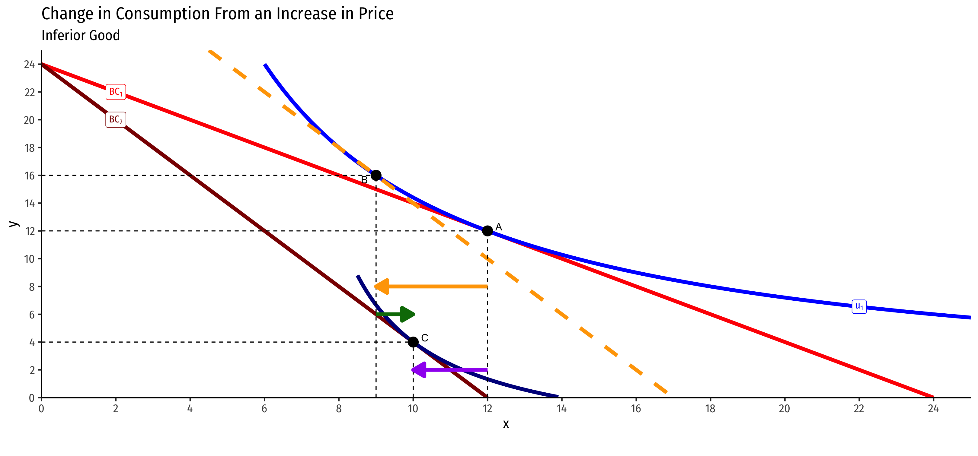
What About Inferior Goods?
Inferior Goods, Graphically I
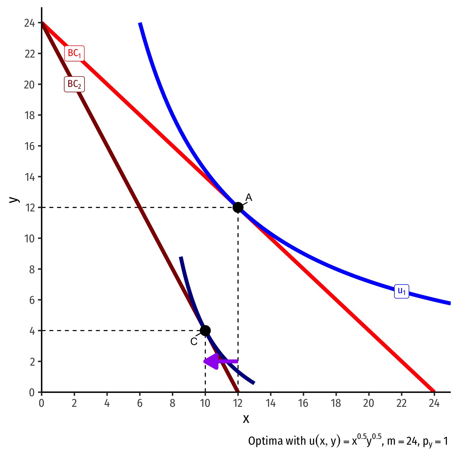
- Original optimal consumption (A)

Inferior Goods, Graphically I
Original optimal consumption (A)
(Total) price effect: A→C
Let's decompose this into the two effects
Inferior Goods, Graphically II
- Substitution effect: what you would choose under the new exchange rate to remain indifferent as before the change

Inferior Goods, Graphically II
Substitution effect: what you would choose under the new exchange rate to remain indifferent as before the change
Graphically: shift new budget constraint inwards until tangent with old indifference curve
A→B on same I.C. (↓ x, ↑ y)

Inferior Goods, Graphically III
- (Real) income effect: change in consumption due to the change in purchasing power from the price change
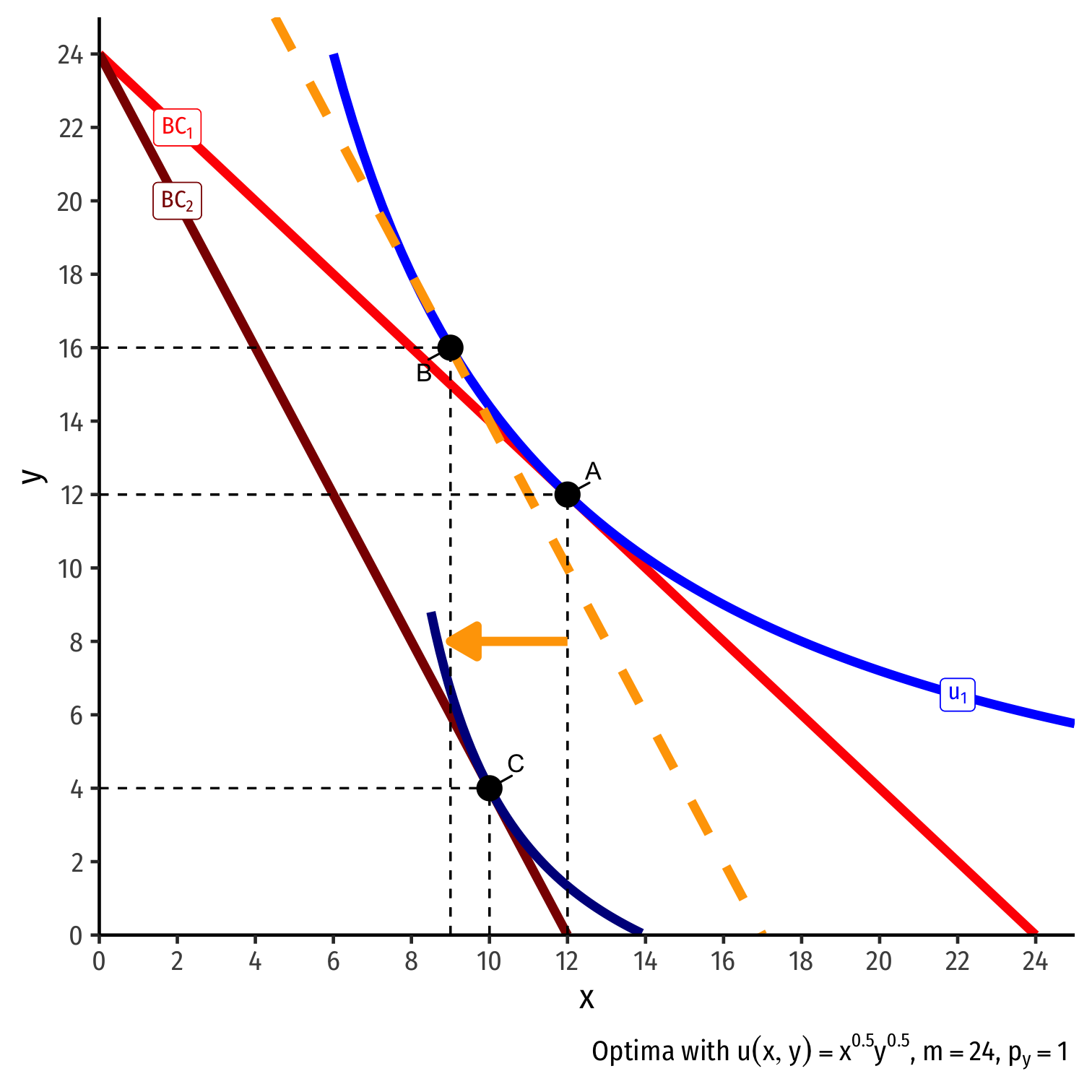
Inferior Goods, Graphically III
(Real) income effect: change in consumption due to the change in purchasing power from the price change
B→C to new budget constraint (can buy less of x and/or y)

Inferior Goods, Graphically IV
- Original optimal consumption (A)
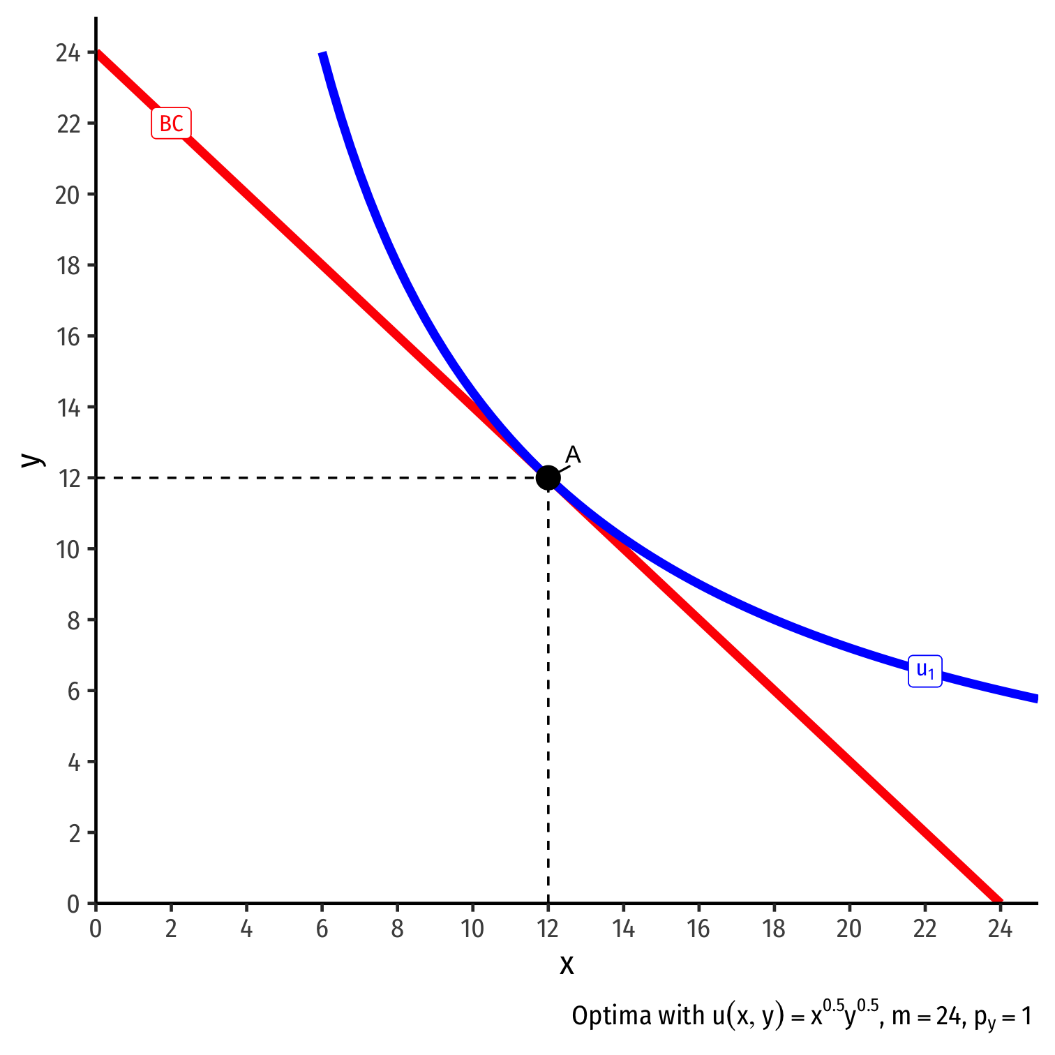
Inferior Goods, Graphically IV
Original optimal consumption (A)
Price of x rises, new optimal consumption at (C)

Inferior Goods, Graphically IV
Original optimal consumption (A)
Price of x rises, new optimal consumption at (C)
Substitution effect: A→B on same I.C. (↓ more expensive x and ↑ y)

Inferior Goods, Graphically IV
Original optimal consumption (A)
Price of x rises, new optimal consumption at (C)
Substitution effect: A→B on same I.C. (↓ more expensive x and ↑ y)
(Real) income effect: B→C to new budget constraint (can buy less x and/or y)
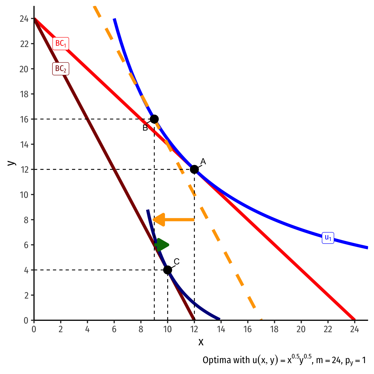
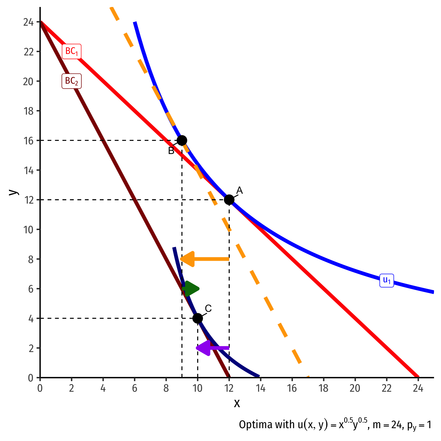
Inferior Goods, Graphically IV
Original optimal consumption (A)
Price of x rises, new optimal consumption at (C)
Substitution effect: A→B on same I.C. (↓ more expensive x and ↑ y)
(Real) income effect: B→C to new budget constraint (can buy less x and/or y)
(Total) price effect: A→C
Violating the Law of Demand
Example: What would it take to violate the law of demand?
A Giffen Good
- Giffen good: theoretical good that violates law of demand
(negative) real income effect > substitution effect
- Few substitutes (small substitution effect)
- An inferior good (negative real income effect)
- A large portion of income spent on it (large real income effect)
- Price increase (decrease) causes person to buy more (less)

Recap: Real Income and Substitution Effects
Price Effect = Real income effect + Substitution Effect
Substitution effect: is always in the direction of the cheaper good
Real Income effect: can be positive (normal) or negative (inferior)
Law of Demand/Demand curves slope downwards (Price effect) mostly because of the substitution effect
- Even (inferior) goods with negative real income effects overpowered by substitution effect
Theoretical Giffen good exception: negative R.I.E. > S.E.
On To Demand Curves
Deriving a Demand Curve Graphically
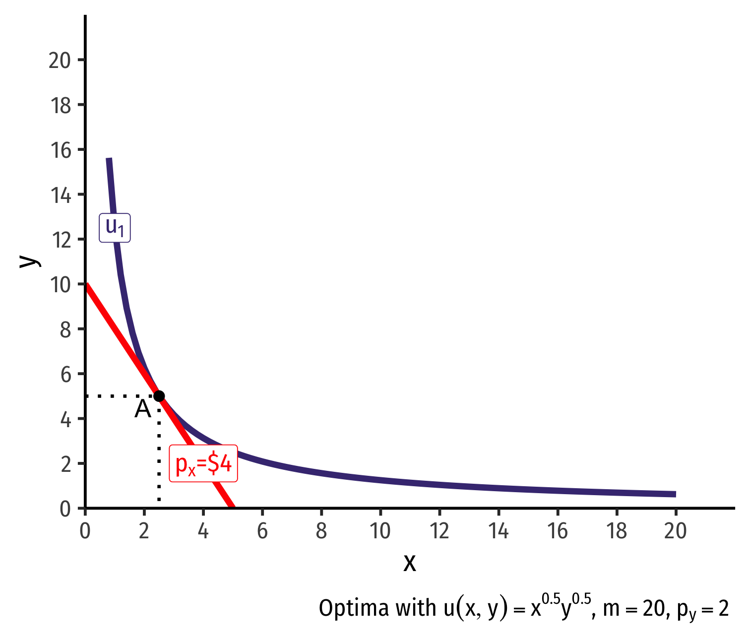
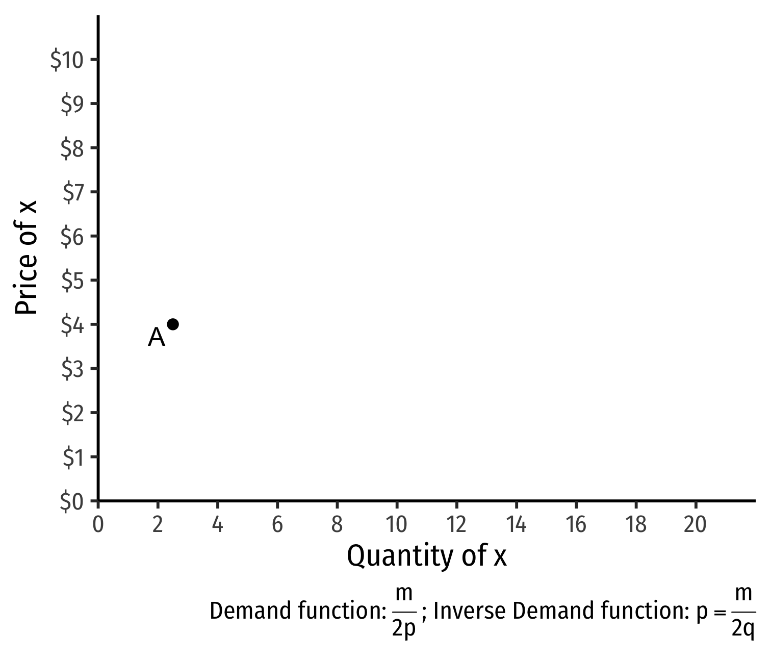
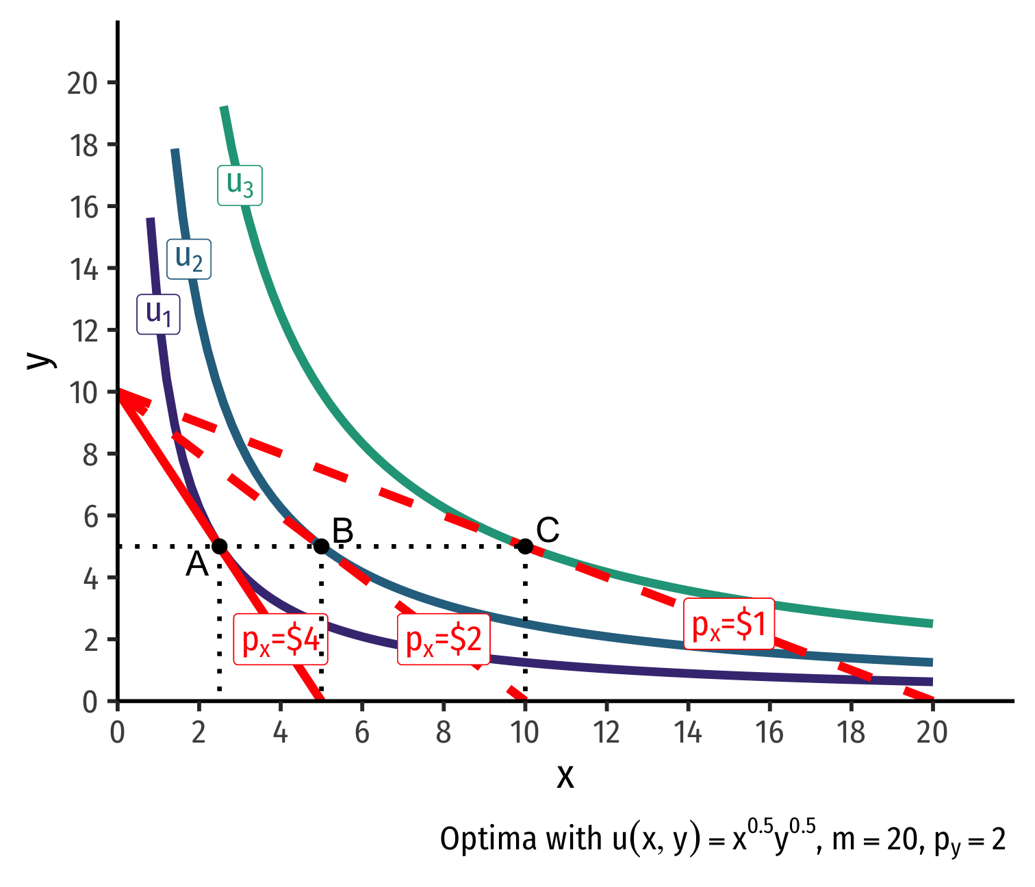
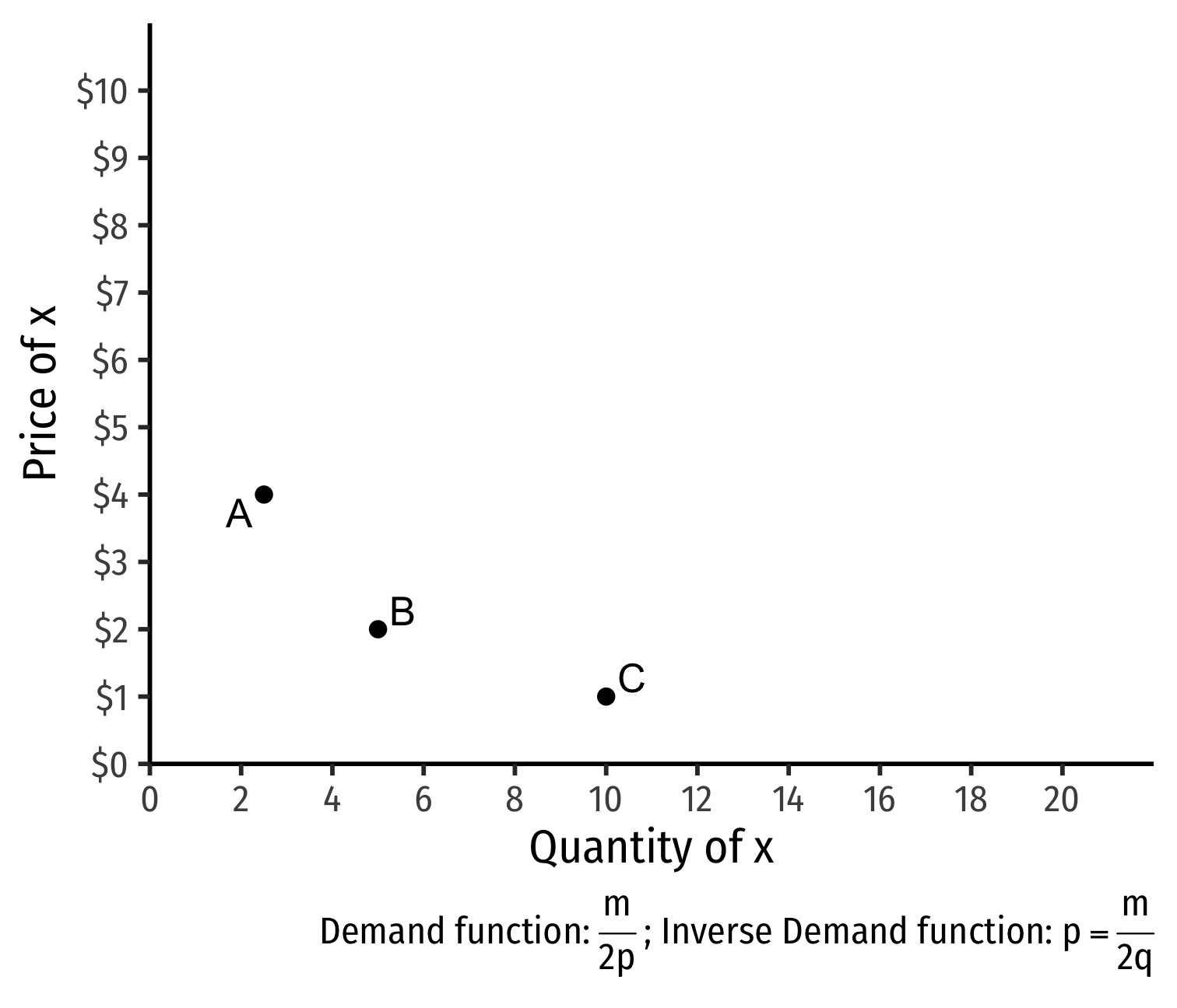
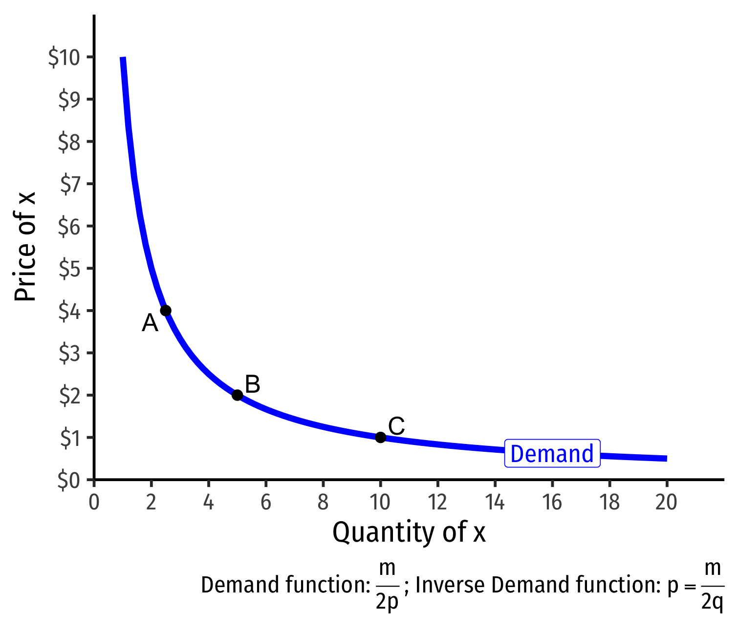
- Demand curve for x relates optimal consumption of x ("quantity") as price of x changes
- At px=4, consumer buys 2 x
Deriving a Demand Curve Graphically
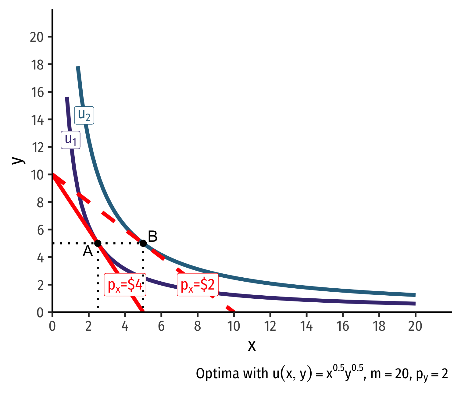

- Demand curve for x relates optimal consumption of x ("quantity") as price of x changes
- At px=4, consumer buys 2 x; at px=2, consumer buys 5 x
Deriving a Demand Curve Graphically
- Demand curve for x relates optimal consumption of x ("quantity") as price of x changes
- At px=4, consumer buys 2 x; at px=2, consumer buys 5 x; at px=1, consumer buys 10 x
Deriving a Demand Curve Graphically

- Demand curve for x relates optimal consumption of x ("quantity") as price of x changes
- At px=4, consumer buys 2 x; at px=2, consumer buys 5 x; at px=1, consumer buys 10 x
From Individual Demand to Market Demand
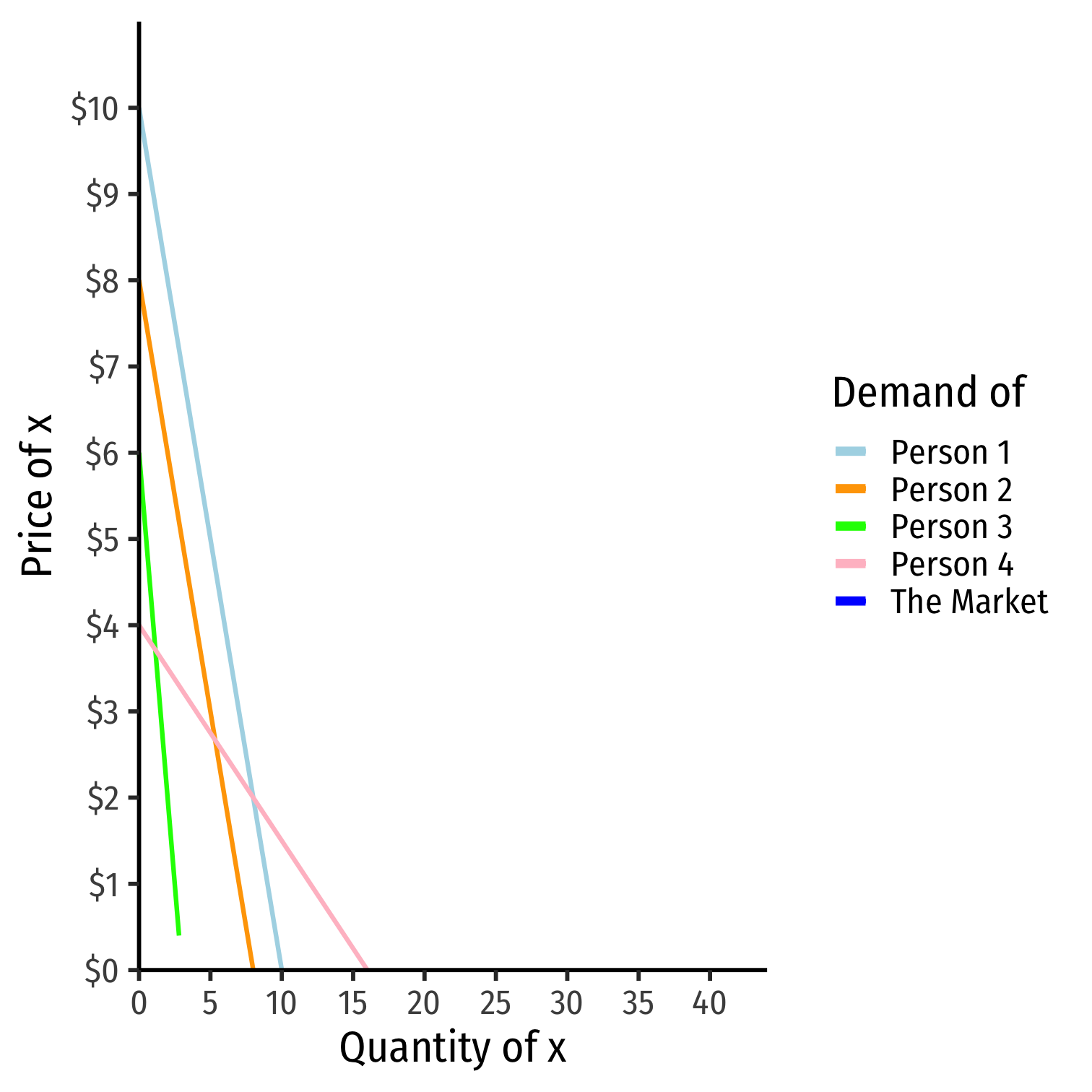
Note so far we have been talking about an individual person’s demand
In principles, you learned about the entire market demand
From Individual Demand to Market Demand
Note so far we have been talking about an individual person’s demand
In principles, you learned about the entire market demand
This is simply the sum of all individuals’ demands
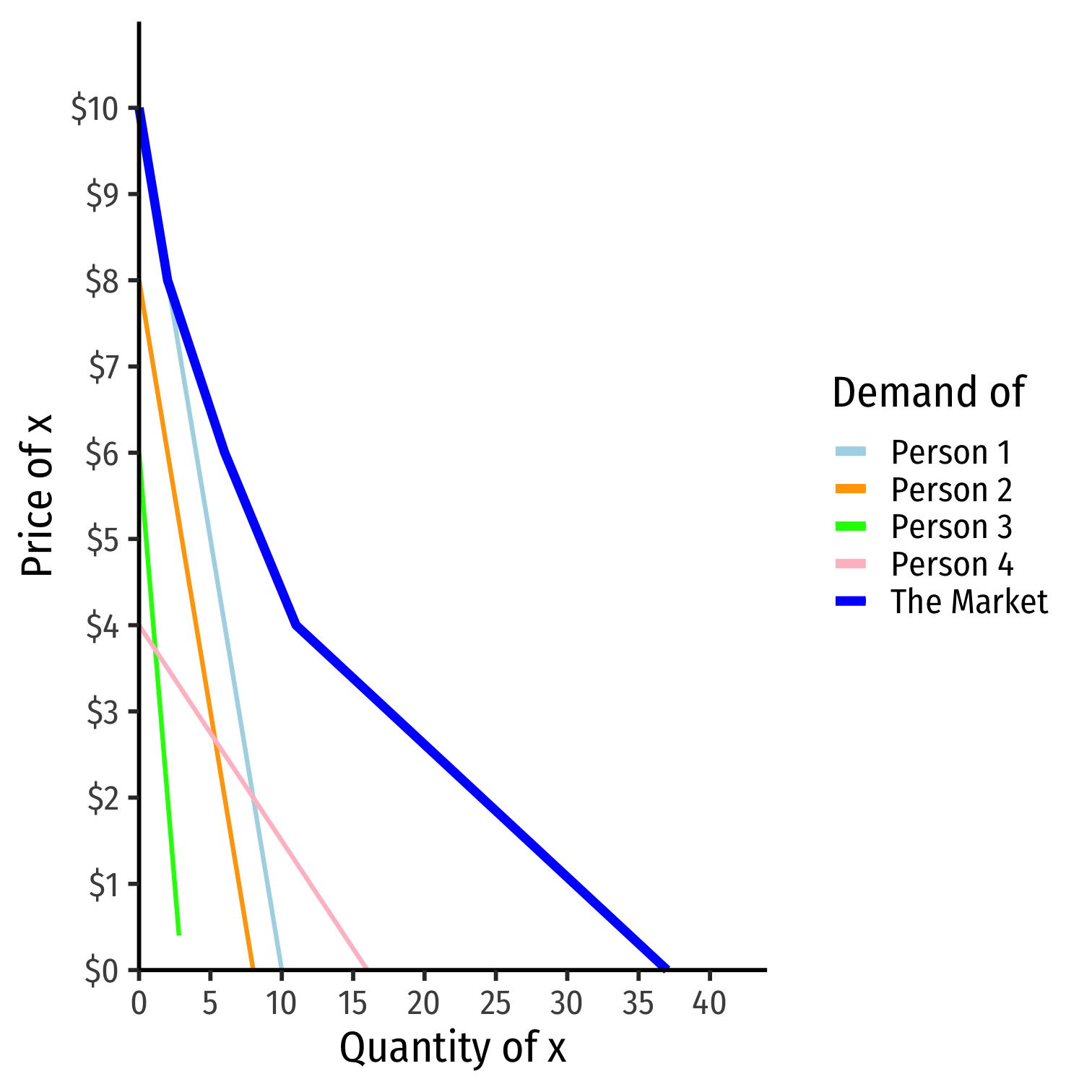
Demand Schedule (For Individual Or Market)
Demand schedule expresses the quantity of good a person(s) would be willing to buy (qD) at any given price (px)
- Holding constant all other prices (py) and income (m)! (“ceterus paribus”)
Note: each of these is a consumer's optimum at a given price!
| price | quantity |
|---|---|
| 10 | 0 |
| 9 | 1 |
| 8 | 2 |
| 7 | 3 |
| 6 | 4 |
| 5 | 5 |
| 4 | 6 |
| 3 | 7 |
| 2 | 8 |
| 1 | 9 |
| 0 | 10 |
Demand Curve
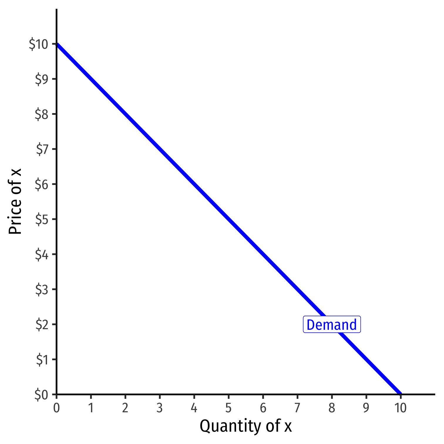
Demand curve graphically represents the demand schedule
Also measures a person's maximum willingness to pay (WTP) for a given quantity
Law of Demand (price effect) ⟹ demand curves always slope downwards

Demand Function
- Demand function relates quantity to price
Example: q=10−p
- Not graphable (wrong axes)!
Inverse Demand Function
- Inverse demand function relates price to quantity
- Take demand function and solve for p
Example: p=10−q
- Graphable (price on vertical axis)!

Inverse Demand Function
- Inverse demand function relates price to quantity
- Take demand function and solve for p
Example: p=10−q
- Vertical intercept ("Choke price"): price where qD=0 ($10), just high enough to discourage any purchases
Inverse Demand Function
Read two ways:
Horizontally: at any given price, how many units person wants to buy
Vertically: at any given quantity, the maximum willingness to pay (WTP) for that quantity
- This way will be very useful later

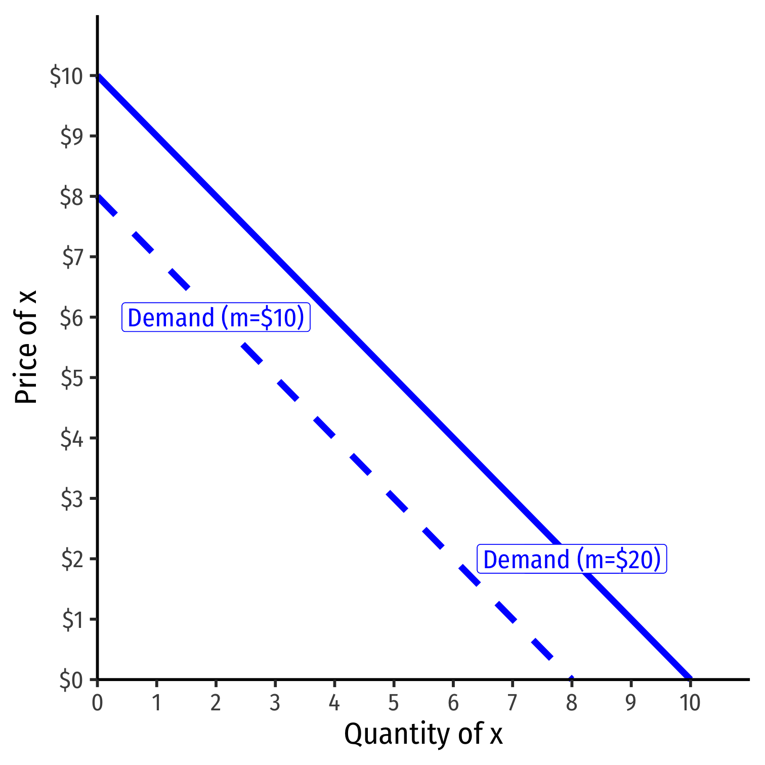
Shifts in Demand I
- Note a simple (inverse) demand function only relates (own) price and quantity
Example: q=10−p or p=10−q
What about all the other "determinants of demand" like income and other prices?
They are captured in the vertical intercept (choke price)!

Shifts in Demand II
A change in one of the "determinants of demand" will shift demand curve!
- Change in income m
- Change in price of other goods py
- Change in preferences or expectations about good x
Shows up in (inverse) demand function by a change in intercept (choke price)!
See my Visualizing Demand Shifters
