1.5 — Demand
ECON 306 • Microeconomic Analysis • Fall 2022
Ryan Safner
Associate Professor of Economics
safner@hood.edu
ryansafner/microF22
microF22.classes.ryansafner.com
The consumer’s Problem: Review
We now can explore the dynamics of how individuals optimally respond to changes in their constraints
We know the (static) problem is:
Choose: < a consumption bundle >
In order to maximize: < utility >
Subject to: < income and market prices >

A Demand Function (for Good X)
- A consumer’s demand (for good x) depends on current prices & income:
qDx=qDx(m,px,py)
- How does demand (for x) change?

A Demand Function (for Good X)
- A consumer’s demand (for good x) depends on current prices & income:
qDx=qDx(m,px,py)
- How does demand (for x) change?
- Income effects (ΔqDxΔm): how qDx changes with changes in income

A Demand Function (for Good X)
- A consumer’s demand (for good x) depends on current prices & income:
qDx=qDx(m,px,py)
- How does demand (for x) change?
- Income effects (ΔqDxΔm): how qDx changes with changes in income
- Cross-price effects (ΔqDxΔpy): how qDx changes with changes in prices of other goods (e.g. y)
- (Own) Price effects (ΔqDxΔpx): how qDx changes with changes in price (of x)

Income Effect
Income Effect
- Income effect: change in optimal consumption of a good associated with a change in (nominal) income, holding relative prices constant
ΔqDΔm>?<0

Income Effect (Normal)
- Consider football tickets and vacation days
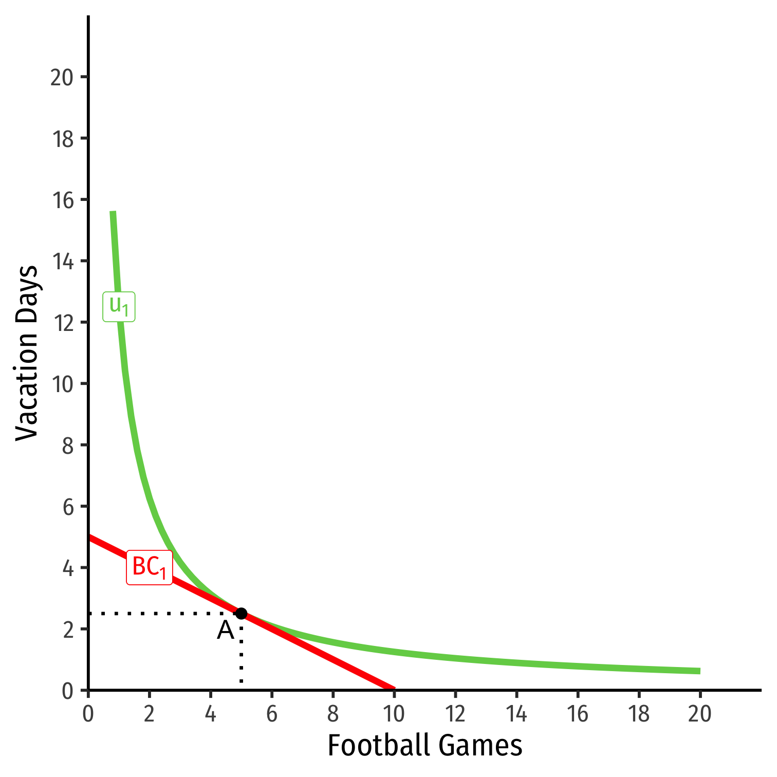
Income Effect (Normal)
Consider football tickets and vacation days
Suppose income (m) increases
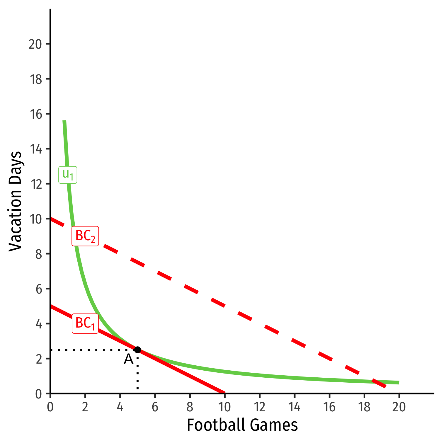
Income Effect (Normal)
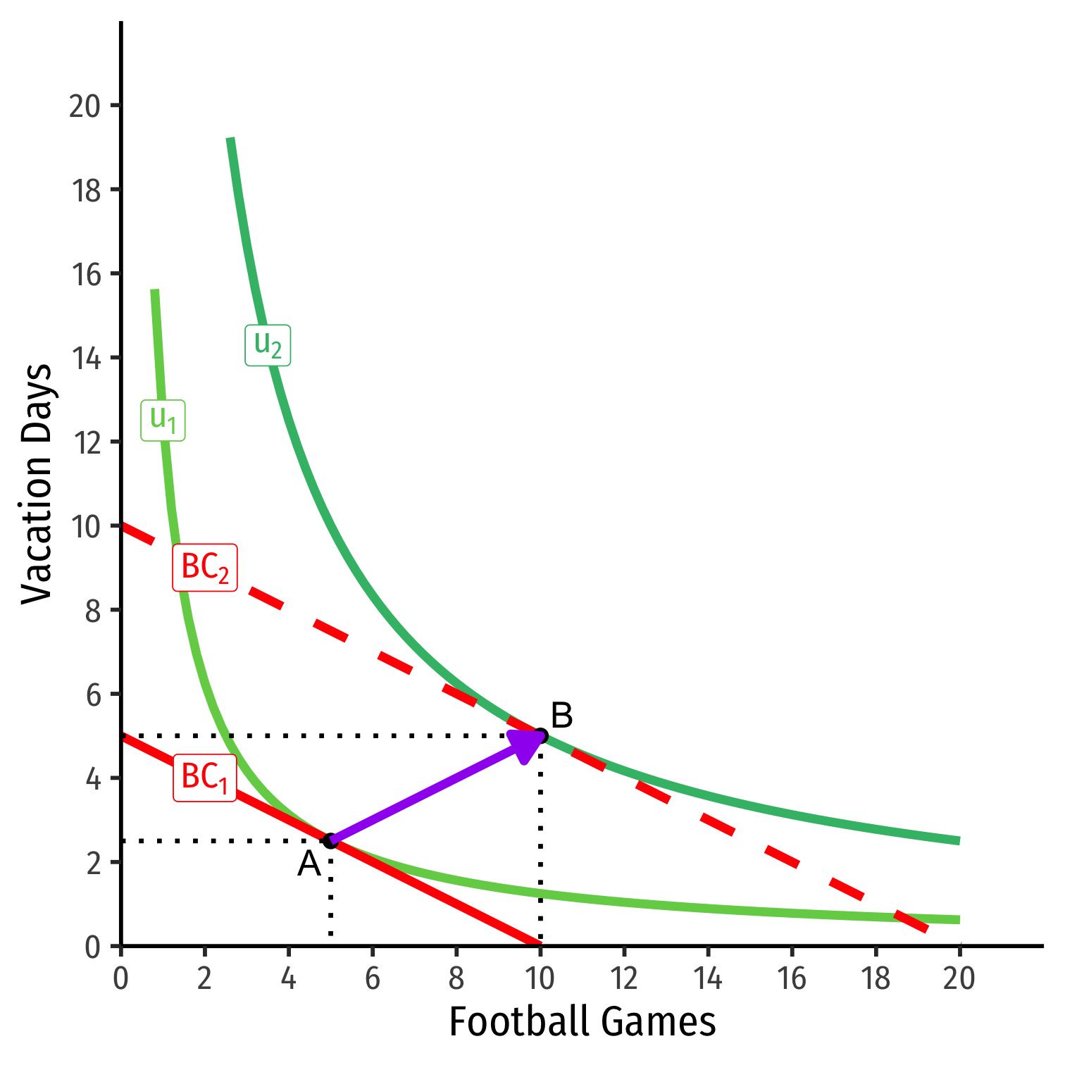
Consider football tickets and vacation days
Suppose income (m) increases
At new optimum (B), consumes more of both
Then both goods are normal goods
Income Effect (Inferior)
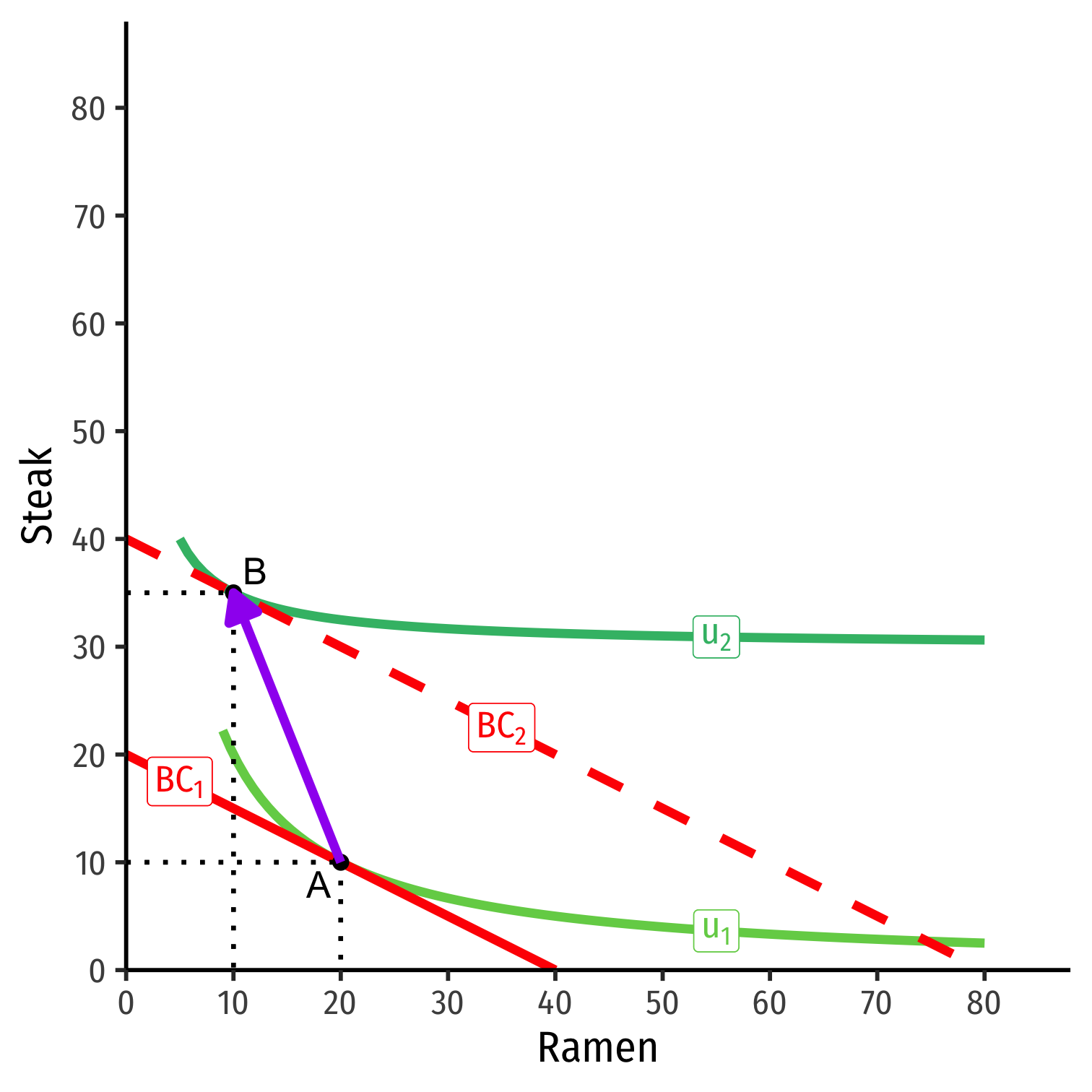
- Consider ramen and steak
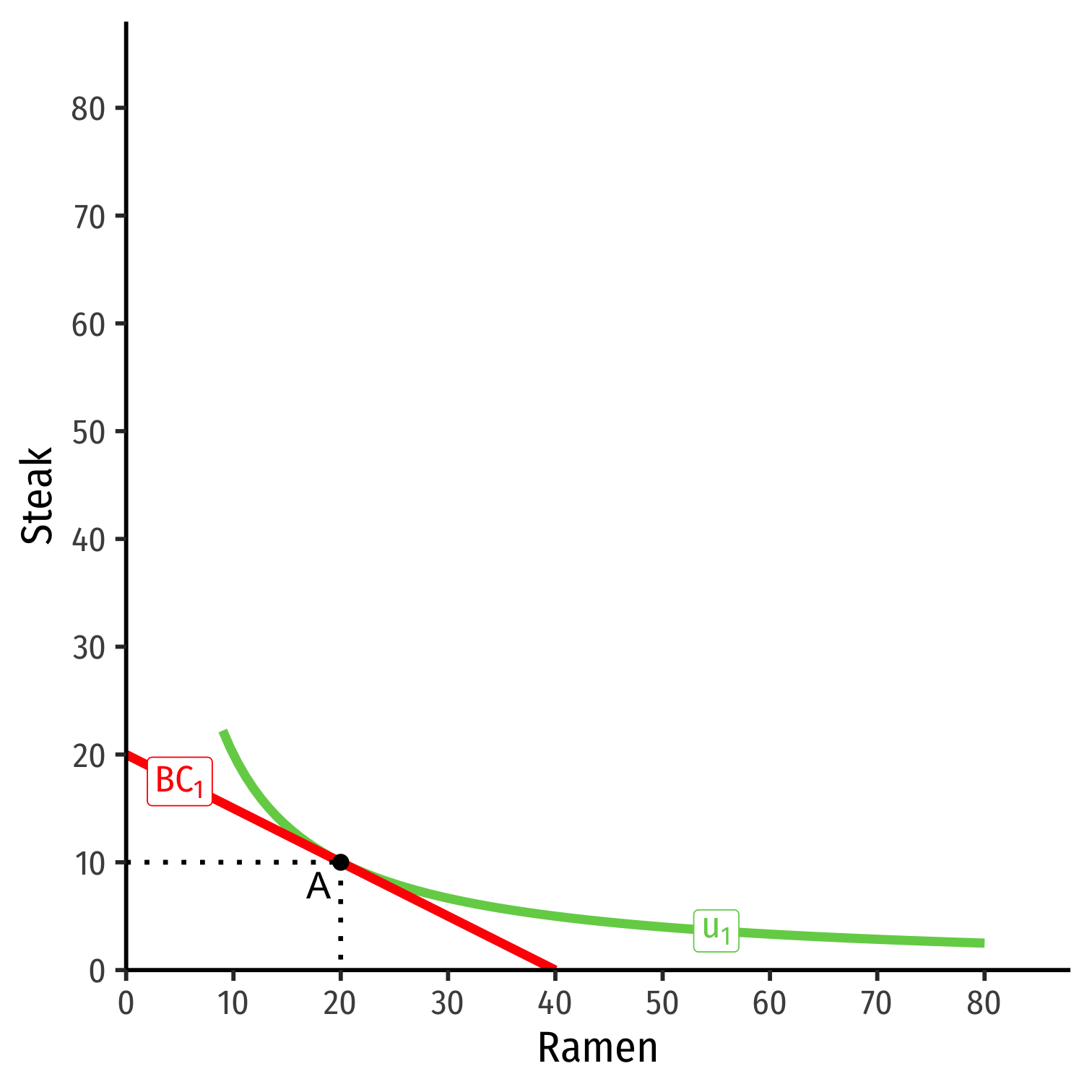
Income Effect (Inferior)
Consider ramen and steak
Suppose income (m) increases
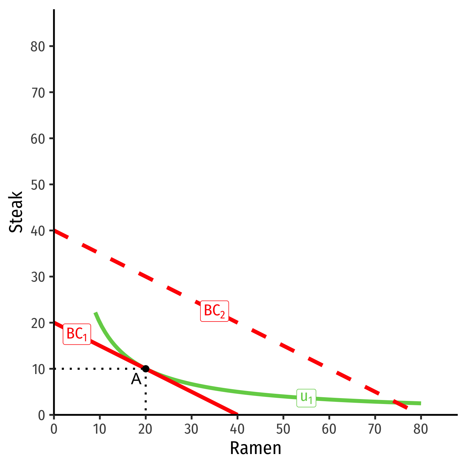
Income Effect (Inferior)
Consider ramen and steak
Suppose income (m) increases
At new optimum (B), consumes more steak, less ramen
Steak is a normal good, ramen is an inferior good
Income Effect
ΔqDΔm>?<0
Normal goods: consumption increases with more income (and vice versa)
Inferior goods: consumption decreases with more income (and vice versa)

Digression: Measuring Change
Quantifying Changes I
Several ways we can talk about how a measure changes over time, from time t1→t2
Difference (Δ): the difference between the value at time t1 and time t2 Δt=t2−t1
Quantifying Changes II
Several ways we can talk about how a measure changes over time, from time t1→t2
Difference (Δ): the difference between the value at time t1 and time t2 Δt=t2−t1
Relative Difference: the difference expressed in terms of the original value Δtt1=t2−t1t1 this becomes a proportion (a decimal)
Quantifying Changes III
- Percentage Change (Growth Rate): relative difference expressed as a percentage
%Δ=Δtt1×100%=t2−t1t1×100%
A Simple Example Growth Rate
Example: A country's GDP is $100bn in 2021, and $120bn in 2022 Calculate the country's GDP growth rate for 2022:
Elasticity, in General
ϵy,x=%Δy%Δx=ΔyyΔxx
- An elasticity between any two variables y and x describes the responsiveness of a variable (y) to a change in another (x).
- (relative change in y) over (relative change in x)
Elasticity, in General
ϵy,x=%Δy%Δx=ΔyyΔxx
An elasticity between any two variables y and x describes the responsiveness of a variable (y) to a change in another (x).
- (relative change in y) over (relative change in x)
Interpretation: ϵy,x= the percentage change in y from a 1% change in x
Elasticity, in General
ϵy,x=%Δy%Δx=ΔyyΔxx
An elasticity between any two variables y and x describes the responsiveness of a variable (y) to a change in another (x).
- (relative change in y) over (relative change in x)
Interpretation: ϵy,x= the percentage change in y from a 1% change in x
Unitless: easy comparisons between any 2 variables
- e.g. crime rates and police, GDP and gov't spending, inequality and corruption
Income Elasticity of Demand I
- The income elasticity of demand measures how much quantity demanded (qD) changes in response to a change in income (m)
ϵq,m=%ΔqD%Δm
Income Elasticity of Demand I
- The income elasticity of demand measures how much quantity demanded (qD) changes in response to a change in income (m)
ϵq,m=%ΔqD%Δm
- If ϵq,m is negative: an inferior good
Income Elasticity of Demand I
- The income elasticity of demand measures how much quantity demanded (qD) changes in response to a change in income (m)
ϵq,m=%ΔqD%Δm
- If ϵq,m is negative: an inferior good
- If ϵq,m is positive: a normal good
Income Elasticity of Demand I
- The income elasticity of demand measures how much quantity demanded (qD) changes in response to a change in income (m)
ϵq,m=%ΔqD%Δm
- If ϵq,m is negative: an inferior good
- If ϵq,m is positive: a normal good
- Two subtypes of normal goods:
- Necessity: 0≤ϵq,m≤1
- ↑ quantity demanded as ↑↑ income (water, clothing)
- Necessity: 0≤ϵq,m≤1
Income Elasticity of Demand I
- The income elasticity of demand measures how much quantity demanded (qD) changes in response to a change in income (m)
ϵq,m=%ΔqD%Δm
- If ϵq,m is negative: an inferior good
- If ϵq,m is positive: a normal good
- Two subtypes of normal goods:
- Necessity: 0≤ϵq,m≤1
- ↑ quantity demanded as ↑↑ income (water, clothing)
- Luxury: ϵq,m>1
- ↑↑ quantity demanded as ↑ income (jewelry, vacations)
- Necessity: 0≤ϵq,m≤1
Income Elasticity of Demand II
- For now, we can calculate the income elasticity of demand simply by calculating the relative changes:
%Δq%Δm=(Δqq1)(Δmm1)
- We'll use some fancier methods when we talk about the only elasticity you've probably seen before: price elasticity of demand
Income Elasticity of Demand: Example
Example: You can spend your income on golf and pancakes. Green fees at a local golf course are $10 per round and pancake mix is $2 per box. When your income is $100, you buy 5 boxes of pancake mix and 9 rounds of golf. When your income increases to $120, you buy 10 boxes of pancake mix and 10 rounds of golf.
What type of good is golf (inferior, necessity, luxury)?
What type of good are pancakes (inferior, necessity, or luxury)?
Income Effects: Example
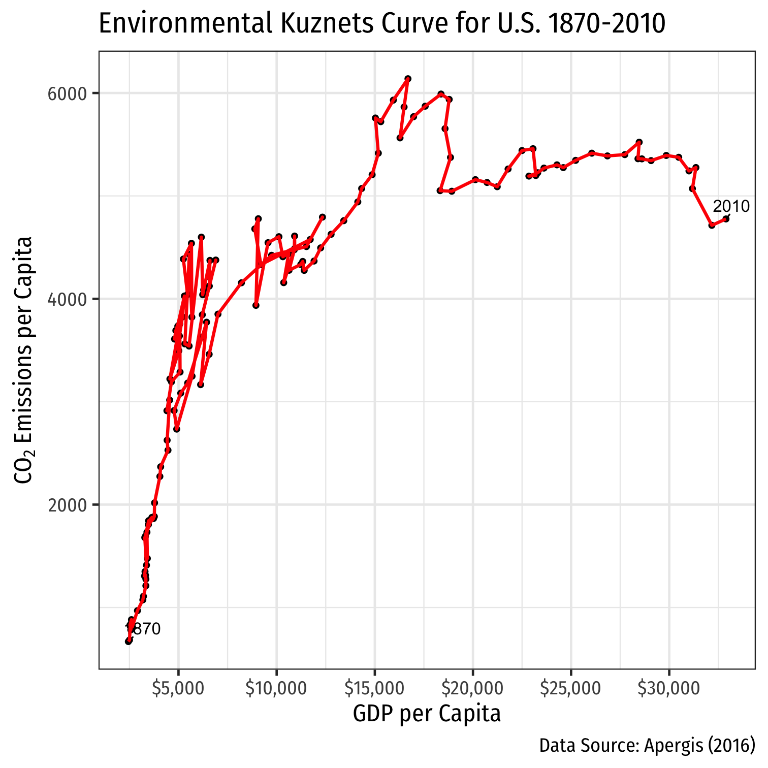
Example: Is the environment a normal good?
Income Effects: Example
Example: Is the environment a normal good?
Income Effects: Example
Example: Is the environment a normal good?

Engel Curves
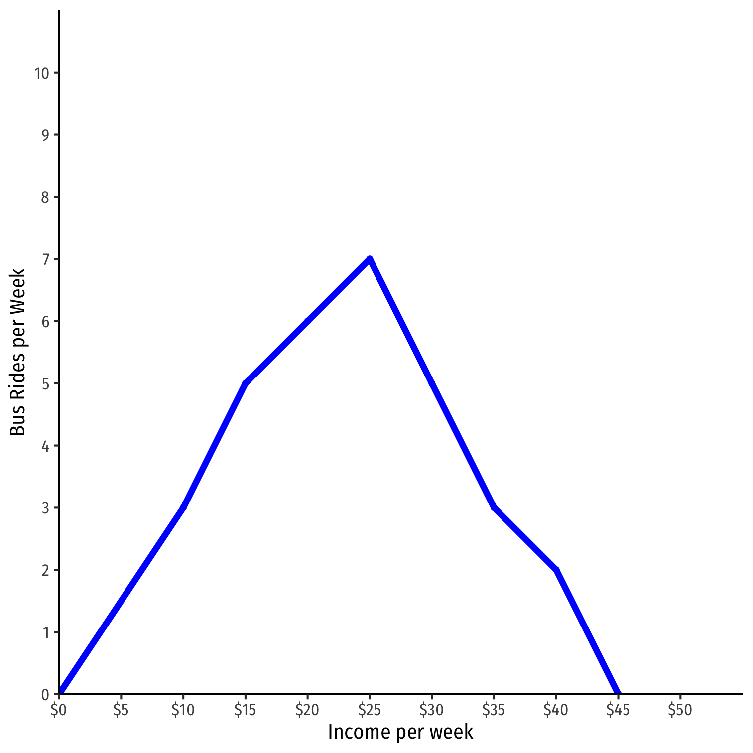
Engel curve visualizes income effects: shows how consumption of one good changes when income increases
When positively sloped: normal good
When negatively sloped: inferior good
Cross-Price Effects
Cross-Price Effects
- Cross-price effect: change in optimal consumption of a good associated with a change in price of another good income, holding the good's own price (and income) constant
ΔqxΔpy>?<0

Cross-Price Elasticity of Demand I
- The cross-price elasticity of demand measures how much quantity demanded of one good (qx) changes in response to a change in price of another good (py)
ϵqx,py=%Δqx%Δpy

Cross-Price Elasticity of Demand I
- The cross-price elasticity of demand measures how much quantity demanded of one good (qx) changes in response to a change in price of another good (py)
ϵqx,py=%Δqx%Δpy=ΔqxqxΔpypy

Cross-Price Elasticity of Demand II
ϵqx,py=%Δqx%Δpy
If ϵqx,py is positive: goods x and y are substitutes
An rise (fall) in price of y causes more (less) consumption of x
- Consumption of x moves in same direction as price of y

Cross-Price Elasticity of Demand III
ϵqx,py=%Δqx%Δpy
If ϵqx,py is negative: goods x and y are complements
Goods x and y consumed in a bundle, concern about overall price of bundle
A rise (fall) in price of y causes less (more) consumption of x
- Consumption of x moves in opposite direction as price of y

Cross-Price Elasticity: Example I
Example: You can travel into the city every week on Lyft rides and Uber rides. When Lyft is $20/ride, you ride 10 Uber rides. When Lyft raises prices to $25/ride, you ride 15 Uber rides.
What is the relationship between these two goods?
What is the cross-price elasticity?